02 - Augmentations, metrics, transfer learning, and experiments tracking
Advanced Image Processing
Poznan University of Technology, Institute of Robotics and Machine Intelligence
![]()
Laboratory 2: Metrics, augmentations, transfer learning, and experiments tracking
Introduction
Building a machine learning model is more than just defining layers and calling a training function. To create a solution that is robust, reliable, and performs well on real-world data, we must adopt a more professional and systematic workflow. This laboratory focuses on the essential techniques that bridge the gap between a simple prototype and a high-performing system.
In this laboratory, we will cover:
metrics - quantitative scores for measuring, comparing, and evaluating a model’s performance.
augmentations - simple yet effective technique to extend dataset, reduce overfitting and improve a model’s ability to generalize,
transfer learning - machine learning technique where a model developed for one task is reused as the starting point for a second, related task,
experiments tracking - the practice of systematically logging and managing all relevant information from model training runs (e.g., hyperparameters, metrics, code), ensuring that every result is organized, comparable, and reproducible.
Goals
The objectives of this laboratory are to:
- understand different metrics, in particular classification metrics,
- familiarize with the concept of image augmentation,
- get to know the concept of transfer learning and why it is useful,
- learn how to track machine learning experiments.
Prerequisites
Install dependencies
PyTorch
pip3 install torch torchvision --index-url https://download.pytorch.org/whl/cu126Lightning
pip install lightningImport libraries
import lightning as L
import torch
import torch.nn as nn
import torch.optim as optim
import torchvision.models as models
import torchvision.transforms as transforms
from torchvision.datasets import OxfordIIITPet
from torch.utils.data import DataLoader
Load dataset
# Define transformations
transform = transforms.Compose([
    transforms.Resize((224, 224)),
    transforms.ToTensor(),
    transforms.Normalize(mean=[0.485, 0.456, 0.406], std=[0.229, 0.224, 0.225])
])

# Load the OxfordIIITPet dataset
train_dataset = OxfordIIITPet(root='./data', split='trainval', download=True, transform=transform)
test_dataset = OxfordIIITPet(root='./data', split='test', download=True, transform=transform)

print(f"Number of training samples: {len(train_dataset)}")
print(f"Number of test samples: {len(test_dataset)}")
💥 Task 1 💥
Add validation dataset and create data loaders.
Load ResNet-18 model
OxfordIIITPet dataset contains 37 classes.
# Load ResNet-18 model
resnet18 = models.resnet18(weights=None)
resnet18.fc = nn.Linear(resnet18.fc.in_features, 37)
Create Lightning-based class for ResNet-18
class LitResNet18(L.LightningModule):
    def __init__(self, model, num_classes: int, learning_rate: float = 1e-3):
        super().__init__()
        self.save_hyperparameters(ignore=['model'])
        self.model = model
        self.loss = nn.CrossEntropyLoss()

        # Buffers to store running totals for correct predictions and total samples.
        self.register_buffer("train_correct", torch.tensor(0.0))
        self.register_buffer("train_total", torch.tensor(0.0))
        self.register_buffer("val_correct", torch.tensor(0.0))
        self.register_buffer("val_total", torch.tensor(0.0))
        self.register_buffer("test_correct", torch.tensor(0.0))
        self.register_buffer("test_total", torch.tensor(0.0))

    def forward(self, x):
        return self.model(x)

    def training_step(self, batch, batch_idx):
        # Reset counters on the first batch of each training epoch
        if batch_idx == 0:
            self.train_correct = self.train_correct.new_zeros(1)
            self.train_total = self.train_total.new_zeros(1)

        x, y = batch
        y_hat = self.model(x)
        loss = self.loss(y_hat, y)

        preds = torch.argmax(y_hat, dim=1)
        self.train_correct += (preds == y).sum()
        self.train_total += y.size(0)

        acc = self.train_correct.float() / self.train_total
        self.log("train_loss", loss)
        self.log("train_acc", acc, on_step=False, on_epoch=True, prog_bar=True)
        return loss

    def validation_step(self, batch, batch_idx):
        # Reset counters on the first batch of each validation epoch
        if batch_idx == 0:
            self.val_correct = self.val_correct.new_zeros(1)
            self.val_total = self.val_total.new_zeros(1)

        x, y = batch
        y_hat = self.model(x)
        loss = self.loss(y_hat, y)

        preds = torch.argmax(y_hat, dim=1)
        self.val_correct += (preds == y).sum()
        self.val_total += y.size(0)

        acc = self.val_correct.float() / self.val_total
        self.log("val_loss", loss, prog_bar=True)
        self.log("val_acc", acc, on_step=False, on_epoch=True, prog_bar=True)

    def test_step(self, batch, batch_idx):
        # Reset counters on the first batch of the test run
        if batch_idx == 0:
            self.test_correct = self.test_correct.new_zeros(1)
            self.test_total = self.test_total.new_zeros(1)

        x, y = batch
        y_hat = self.model(x)
        loss = self.loss(y_hat, y)

        preds = torch.argmax(y_hat, dim=1)
        self.test_correct += (preds == y).sum()
        self.test_total += y.size(0)

        acc = self.test_correct.float() / self.test_total
        self.log("test_loss", loss, prog_bar=True)
        self.log("test_acc", acc, on_step=False, on_epoch=True, prog_bar=True)

    def configure_optimizers(self):
        optimizer = optim.AdamW(self.parameters(), lr=self.hparams.learning_rate)
        return optimizer
Wrap it into the Lightning training pipeline.
# Initialize the model and trainer
model = LitResNet18(resnet18, num_classes=37)

trainer = L.Trainer(max_epochs=10)
trainer.fit(model, train_dataloaders=train_dataloader, val_dataloaders=val_dataloader)
trainer.test(model, test_dataloader)
Train the model and verify it performance on the test set.
Metrics
In deep learning, and in general in machine learning, metrics are the essential tools for measuring, comparing, and improving the performance of models. They provide a quantitative score that inform how well a model is performing its task, translating complex predictions into a simple, understandable number.
Types of metrics
The choice of evaluation metric is fundamentally tied to the specific task a machine learning model is designed to solve. Different tasks have distinct goals, and therefore, require different ways of measuring success. Metrics can be broadly categorized based on the machine learning (computer vision) task they are intended to evaluate. The below metrics are only examples.
- Classification:
- Accuracy - represents the ratio of correct predictions to the total number of predictions.
- Precision - measures model’s exactness - a high precision means that the model has a low false positive rate.
- Recall (Sensitivity or True Positive Rate) - measures model’s completeness - a high recall means that the model has a low false negative rate.
- F1-Score - the harmonic mean of precision and recall, useful when you need to consider both false positives and false negatives.
- Regression:
- Mean Absolute Error (MAE) - the average of the absolute differences between the predicted and actual values.
- Mean Squared Error (MSE) - the average of the squared differences between the predicted and actual values.
- Segmentation:
- Dice Score - measures the similarity between two sets, most commonly to evaluate the overlap between a predicted segmentation mask and a ground truth mask.
- Object detection:
- Intersection over Union (IoU) - the foundational metric that measures how much a predicted bounding box overlaps with the ground truth box.
- Mean Average Precision (mAP) - the gold standard for measuring object detection performance, providing a single number that summarizes a model’s accuracy across all object classes and confidence levels.
Metrics related to segmentation and object detection will be covered in more detail during classes devoted to these tasks.
TorchMetrics
TorchMetrics is a PyTorch-native library that provides a standardized, efficient, and reliable collection of over 100 machine learning metrics. It’s designed to make models evaluation simple and robust. To install TorchMetrics package run:
pip install torchmetrics💥 Task 2 💥
In LitResNet18 implementation replace custom accuracy
calculation with metric from TorchMetrics package. Add also other
classification metrics such as Precision, Recall, and F1-Score. Re-train
model and verify it performance on the test set.
💥 Tips:
Use MetricCollection to simplify implementation.
Use
clonemethod (of class MetricCollection) with prefix parameter to create the same metrics set for train, validation, and test steps.
Augmentations
In machine learning, the performance and generalization ability of a model are heavily dependent on the quality and quantity of the training data. Therefore, data augmentation is a powerful technique used to artificially increase the size and diversity of a training dataset by creating modified, yet plausible, versions of existing data. It’s one of the most effective strategies to combat overfitting and improve model robustness, especially when the amount of available training data is limited.
The core idea is to apply a series of random (but realistic) transformations to the training images. For a model, an image of a cat that is slightly rotated or flipped horizontally is still an image of a cat. By exposing the model to these variations, it learns to recognize the core features of the object, regardless of its orientation, position, or lighting conditions.
Common augmentation techniques for images include:
- Geometric transformations:
- Rotation - rotates the image by a random angle.
- Flipping - flips the image horizontally, vertically or horizontally and vertically.
- Cropping - randomly crops a section of the image.
- Scaling - zooms in or out on the image.
- Translation - shifts the image horizontally or vertically.
- Color and photometric transformations:
- Brightness/contrast adjustment - randomly alter the brightness or contrast.
- Hue/saturation jitter - changes the color properties of the image.
- Additive noise - adds random noise to the image pixels.
By applying these augmentations, it is possible to create a virtually infinite stream of unique training examples from a finite dataset, forcing the model to learn more general and invariant features. This ultimately leads to a more robust model that performs better on new, unseen data.
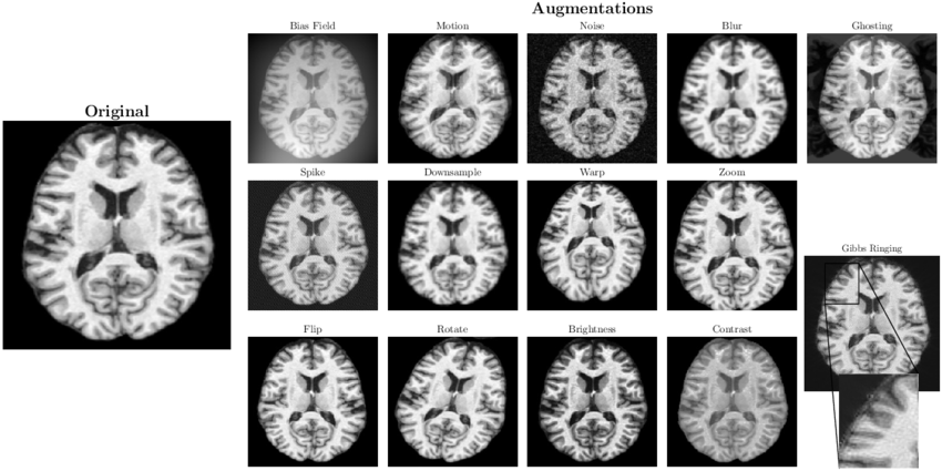
Example augmentations. Images source:
deepmriprep: Voxel-based
Morphometry (VBM) Preprocessing via Deep Neural Networks
💥 Task 3 💥
Using transforms.Compose define augmentations similarly to transformations assigned to transform variable. Select 5 different augmentations and apply them to train dataset instead of transformations.
💥 Tip: Remember to add
transformations from transform to augmentations list.
Transfer learning
Transfer learning is a powerful and popular machine learning technique where a model developed for one task is repurposed as the starting point for a second, related task. Instead of training a model from scratch, which often requires vast amounts of labeled data and significant computational resources, we can leverage knowledge a pre-trained model has already learned.
The core idea is analogous to how humans learn. We don’t start from a blank slate for every new task. For example, knowledge gained from learning to ride a bicycle can be transferred to make it easier to learn how to ride a motorcycle.
In deep learning, this typically involves taking a pre-trained model, such as a ResNet trained on the massive ImageNet dataset, and adapting it to a new, more specific problem. The pre-trained model has already learned to recognize a rich hierarchy of features (like edges, textures, and shapes) from its original training data. We can reuse these learned feature-extraction layers and simply retrain the final classification layers for our specific task, a process known as fine-tuning.
![]()
Transfer learning concept. Image source:
What
is Transfer Learning?
Why Use Transfer Learning?
- Less data required - it vastly reduces the amount of labeled data needed for the new task.
- Faster development - training is much faster since you are only fine-tuning a small part of the network.
- Better performance - it often results in a higher-performing model because the pre-trained model provides a better starting point with robust, generalized features.
💥 Task 4 💥
In code section, where ResNet-18 model is loaded set
weights="IMAGENET1K_V1" and load network with weights
pre-trained on ImageNet dataset. Re-train model and check how it impacts
on model performance.
💥 Task 5 💥
Replace the model initialization with the following code snippet. In this example, all the layers except the final classification layer are frozen.
resnet18 = models.resnet18(weights="IMAGENET1K_V1")
for param in resnet18.parameters():
    param.requires_grad = False

num_classes = 37
num_ftrs = resnet18.fc.in_features
resnet18.fc = nn.Linear(num_ftrs, num_classes)

model = LitResNet18(resnet18, num_classes=num_classes)
Examine how it impacts on model performance. Repeat also the test for
the parameter weights=None.
Experiments tracking
Training a machine learning model is an iterative and often chaotic process. It involves constantly tweaking code, adjusting hyperparameters, changing model architectures, and experimenting with different datasets. Without a systematic approach, it’s easy to lose track of which combination of factors led to a specific result. This is where experiment tracking comes in. In general, experiment tracking is the practice of systematically logging all the important components of the machine learning experiments, ensuring that every result is reproducible, comparable, and easy to analyze. It allows creating a clear, organized history of the work.
Why Is Experiment Tracking Crucial?
Reproducibility - allows perfectly recreating any experiment, ensuring the work is reliable and scientifically sound.
Organization - creates an organized history of a project’s development.
Insight - enables developers to instantly identify which changes to the code or hyperparameters led to better model performance.
Collaboration - creates a transparent and shared project history, making it easy for team members to understand progress, compare results, and build on previous work.
Essentially, you track everything needed to reproduce a result, including:
- hyperparameters (learning rate, batch size, optimizer settings, etc.),
- metrics (e.g., loss, accuracy, F1-score),
- model artifacts (saved model weights, checkpoints, visualizations, plots, etc.),
- code version - the specific Git commit hash of the source code used for the run,
- dataset version - information about the data used for training, validation, and test.
MLflow
MLflow is a specialized tool, designed to automate experiments tracking, providing dashboards to visualize and manage experiments with with little effort and just a few lines of code.
![]()
Image
source: MLflow
💥 Task 6 💥
Install MLflow
pip install mlflowAdd MLflow Logger from lightning package to the training pipeline. Re-train model and observe automated logging and plotting in MLflow dashboard.
💥 Tip: To open
interactive dashboard use mlflow ui command.