04 - Advanced classification with Transformer network
Advanced Image Processing
Poznan University of Technology, Institute of Robotics and Machine Intelligence
![]()
Laboratory 4: Advanced classification with Transformer network
Introduction
For years, Convolutional Neural Networks (CNNs) have been the undisputed champions of computer vision. But what if there’s a different way for a model to “see”? A way inspired not by sliding filters over pixels, but by understanding the relationships between different parts of an image, much like how Transformers revolutionized natural language processing.
In this laboratory, you will learn about new model architecture - the Vision Transformer (ViT). In addition, this notebook introduces other sophisticated topics related to image classification, such as:
- advanced image augmentation techniques (Mixup, Cutout, Cutmix) - to build a more robust model that can handle real-world variations
- label smoothing - a regularization method to prevent our model from becoming overconfident in its predictions
Goals
The objectives of this laboratory are to:
- get hands-on experience in implementing advanced image augmentation techniques,
- understand the concept of label smoothing,
- familiarize with Transformer architecture and its implementation.
References
- mixup: Beyond Empirical Risk Minimization
- Improved Regularization of Convolutional Neural Networks with Cutout
- Cutmix: Regularization strategy to train strong classifiers with localizable features
- Rethinking the Inception Architecture for Computer Vision - label smoothing method description
- An image is worth 16x16 words: Transformers for image recognition at scale - Vision Transformer (ViT) paper
- Vision Transformer (ViT) Architecture
- Building Vision Transformers (ViT) from scratch
Prerequisites
Install dependencies
PyTorch
pip3 install torch torchvision --index-url https://download.pytorch.org/whl/cu126Lightning
pip install lightningLoad dataset
from torchvision import datasets, transforms


def get_dataloaders(batch_size: int = 32):
    # Define transformations
    transform = transforms.Compose([
        transforms.Resize((224, 224)),
        transforms.ToTensor(),
        transforms.Normalize(mean=[0.485, 0.456, 0.406], std=[0.229, 0.224, 0.225]),
    ])

    # Load the OxfordIIITPet dataset
    trainval_dataset = datasets.OxfordIIITPet(root='./data', split='trainval', download=True, transform=transform)
    test_dataset = datasets.OxfordIIITPet(root='./data', split='test', download=True, transform=transform)

    ############# TODO: Student code #####################

    # 1. Split train dataset into train and validation

    # 2. Create data loaders
    train_dataloader = None
    val_dataloader = None
    test_dataloader = None

    ######################################################

    return train_dataloader, val_dataloader, test_dataloader
💥 Task 1 💥
Add validation dataset and create data loaders complementing the above code snippet.
Advanced image augmentation
The application of data augmentations is almost guaranteed to improve the performance of a neural network. Augmentations are a regularization technique that artificially expands the training data and helps the deep learning model generalize better. Consequently, image augmentations have the potential to enhance model performance. Beyond conventional methods such as geometric operations (e.g., flip, rotate, resize, etc.), blurring techniques (e.g., Gaussian, motion blur, etc.), or pixel-based operations (e.g., CLAHE, salt and pepper, color, jitter, etc.), more advanced techniques can be distinguished, such as:
- Mixup - mix a random pair of input images and their labels.
- Cutout - randomly remove a square region of pixels in an input image.
- Cutmix - randomly select a pair of input images, cut a random patch of pixels from the first image and paste it to the second image, and then mix their labels proportionally to the area of the patch.
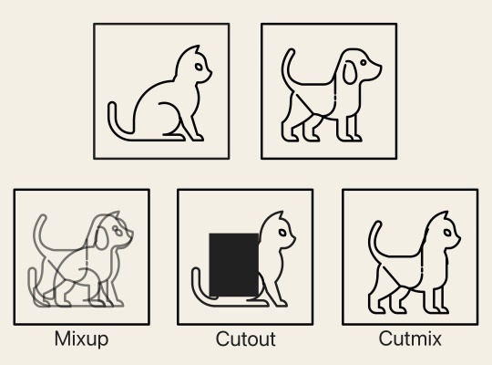
Image source:
towardsdatascience.com
💥 Task 2 💥
Based on the implementation below, test the Cutmix augmentation
method. To do this, follow the instructions and complete the script
snippet by adding the get_dataloaders function and calling
it to obtain train_dataloader.
Run script several times to observe the Cutmix augmentation in action.
cutmix.py
import numpy as np
import torch
from torchvision import datasets, transforms


class Cutmix:
    """Applies Cutmix augmentation to a batch of images and labels.

    Cutmix is a data augmentation technique that involves cutting a patch from one image and pasting it onto another.
    The labels are then mixed proportionally to the area of the patch. The object is called inside the training loop.

    Parameters
    ----------
    alpha : float, default=1.0
        Cutmix hyperparameter for the Beta distribution. This controls the
        distribution of the patch sizes. If alpha is 0, no Cutmix is applied.
    p : float, default=0.5
        The probability of applying the Cutmix augmentation to each sample in a batch.
    """
    def __init__(self, alpha: float = 1.0, p: float = 0.5):
        self.alpha = alpha
        self.p = p

    def _rand_bbox(self, size, lam):
        """Generates a random bounding box."""
        W = size[2]
        H = size[3]
        cut_rat = np.sqrt(1. - lam)
        cut_w = int(W * cut_rat)
        cut_h = int(H * cut_rat)

        # Uniformly sample the center of the box
        cx = np.random.randint(W)
        cy = np.random.randint(H)

        # Calculate box coordinates, clipping to be within image boundaries
        bbx1 = np.clip(cx - cut_w // 2, 0, W)
        bby1 = np.clip(cy - cut_h // 2, 0, H)
        bbx2 = np.clip(cx + cut_w // 2, 0, W)
        bby2 = np.clip(cy + cut_h // 2, 0, H)

        return bbx1, bby1, bbx2, bby2

    def __call__(self, images: torch.Tensor, labels: torch.Tensor):
        """Performs the Cutmix transformation on a batch.

        This method applies Cutmix to each sample in the batch with a probability `self.p`.

        Parameters
        ----------
        images : torch.Tensor
            A batch of images of shape (N, C, H, W).
        labels : torch.Tensor
            A batch of corresponding labels of shape (N,).

        Returns
        -------
        tuple[torch.Tensor, torch.Tensor, torch.Tensor, torch.Tensor]
            A tuple containing:
            - **mixed_images** (*torch.Tensor*): The batch with Cutmix applied.
            - **labels_a** (*torch.Tensor*): The original labels.
            - **labels_b** (*torch.Tensor*): The labels from the shuffled batch corresponding to the pasted patches.
            - **lam_batch** (*torch.Tensor*): A tensor of shape (N,) containing the mixing ratio for each sample.
                                            `lam_batch` is 1.0 for samples where Cutmix was not applied.
        """
        # Return the original batch if augmentation is disabled
        if self.alpha <= 0 or self.p <= 0:
            lam = torch.ones(images.size(0), device=images.device)
            return images, labels, labels, lam

        batch_size, _, H, W = images.shape
        device = images.device

        # Get a shuffled batch for mixing
        index = torch.randperm(batch_size, device=device)
        labels_a, labels_b = labels, labels[index]

        # Initialize outputs
        mixed_images = images.clone()
        lam_batch = torch.ones(batch_size, device=device)

        # Iterate over each sample in the batch
        for i in range(batch_size):
            # Apply Cutmix with probability p
            if torch.rand(1).item() < self.p:
                # 1. Sample lambda from the Beta distribution
                lam = np.random.beta(self.alpha, self.alpha)

                # 2. Generate the bounding box for the patch
                bbx1, bby1, bbx2, bby2 = self._rand_bbox(images.size(), lam)

                # 3. Get the partner image to cut the patch from
                partner_index = index[i]

                # 4. Paste the patch onto the original image
                mixed_images[i, :, bby1:bby2, bbx1:bbx2] = images[partner_index, :, bby1:bby2, bbx1:bbx2]

                # 5. Adjust lambda to match the true patch area and store it
                area = (bbx2 - bbx1) * (bby2 - bby1)
                lam_adjusted = 1.0 - (area / (H * W))
                lam_batch[i] = lam_adjusted

        return mixed_images, labels_a, labels_b, lam_batch


def main():
    ############# TODO: Student code #####################
    # Add above `get_dataloaders` function and call it to get `train_dataloader`


    ######################################################
    # Get a batch of images and labels
    images, labels = next(iter(train_dataloader))

    # Initialize and apply the Cutmix transform
    cutmix_transform = Cutmix(alpha=1.0)
    augmented_images, labels_a, labels_b, lam_batch = cutmix_transform(images, labels)

    # --- Visualization ---
    num_images_to_show = 4

    fig, axes = plt.subplots(1, num_images_to_show, figsize=(4 * num_images_to_show, 5))
    fig.suptitle(f"Cutmix", fontsize=32)

    for i in range(num_images_to_show):
        lam = lam_batch[i]
        # --- Plot the augmented image ---
        mixed_image_np = augmented_images[i].permute(1, 2, 0).numpy()
        # Unnormalize the image
        mean = np.array([0.485, 0.456, 0.406])
        std = np.array([0.229, 0.224, 0.225])
        mixed_image_np = mixed_image_np * std + mean
        # Normalize for display
        mixed_image_np = (mixed_image_np - mixed_image_np.min()) / (mixed_image_np.max() - mixed_image_np.min())

        axes[i].imshow(mixed_image_np)
        axes[i].set_title(f"Labels: {labels_a[i]} & {labels_b[i]} (λ ≈ {lam:.2f})")
        axes[i].axis('off')

    plt.tight_layout(rect=[0, 0, 1, 0.95]) # Adjust layout for the main title
    plt.show()


if __name__ == "__main__":
    main()
💥 Task 3 💥
Based on the above description and illustrative visualization
implement Cutout augmentation method. Follow the instructions placed
inside the source code. Reuse and adjust source code from
cutmix.py to test Cutout augmentation on data from
OxfordIIITPet dataset.
Run script several times to observe the Cutmix augmentation in action.
Note: __call__ method takes a single
image.
Cutout augmentation code template
class Cutout:
    """Applies Cutout augmentation to a batch of images.

    This augmentation randomly masks out one or more square regions of an input image.

    Parameters
    ----------
    n_holes : int
        Number of patches to cut out from an image.
    length : int
        The length (in pixels) of each square patch.
    """
    def __init__(self, n_holes: int, length: int):
        self.n_holes = n_holes
        self.length = length

    def __call__(self, image: torch.Tensor):
        """Applies the cutout transformation.

        Parameters
        ----------
        image : torch.Tensor
            Tensor image of size (C, H, W).

        Returns
        -------
        torch.Tensor
            Image with `n_holes` of dimension `length` x `length` cut out.
        """
        ############# TODO: Student code #####################
        # Step 1: Initialize a single channel mask with all ones (`np.ones`) and input tensor HxW dimensions

        # Create n_holes square patches in the mask
        for _ in range(self.n_holes):
            # Step 2: Randomly select center point for the hole
            # Step 3: Calculate boundaries of the square patch, considering (y, x) as square patch center and `self.length` as patch length
            # Step 4: Clip boundaries of the square patch to image boundaries `np.clip`
            # Step 5: Set the patch region in mask to 0 (black out the region)

        # Step 6: Convert numpy mask to torch tensor
        # Step 7: Add a channel dimension to the mask: (H, W) => (C, H, W)
        # Step 8: Apply mask to image (element-wise multiplication)

        ######################################################

        return image
💥 Task 4 💥
Based on the above description and illustrative visualization
implement Mixup augmentation method. Follow the instructions placed
inside the source code. Reuse and adjust source code from
cutmix.py to test Mixup augmentation on data from
OxfordIIITPet dataset.
Run script several times to observe the Cutmix augmentation in action.
Note: __call__ method takes a batch of
images.
Mixup code template
class Mixup:
    """Applies Mixup to a batch of images and labels.

    Mixup constructs virtual training examples by forming convex combinations of pairs of examples and their labels.
    This technique helps to regularize the model and improve generalization. The object is called inside the training loop.

    Parameters
    ----------
    num_classes : int
        The total number of classes in the dataset.
    alpha : float, default=1.0
        Mixup hyperparameter for the Beta distribution. If alpha is 0,
        no mixup is applied.
    """
    def __init__(self, num_classes: int, alpha: float = 1.0):
        self.num_classes = num_classes
        self.alpha = alpha

    def __call__(self, images: torch.Tensor, labels: torch.Tensor):
        """Performs the Mixup transformation on a batch.

        Parameters
        ----------
        images : torch.Tensor
            A batch of images of shape (N, C, H, W).
        labels : torch.Tensor
            A batch of corresponding labels of shape (N,).

        Returns
        -------
        tuple[torch.Tensor, torch.Tensor]
            A tuple containing:
            - **mixed_images** (*torch.Tensor*): The batch of mixed images.
            - **mixed_labels** (*torch.Tensor*): The batch of mixed, one-hot
              encoded labels.
        """
        if self.alpha <= 0:
            return images, F.one_hot(labels, num_classes=self.num_classes).float()

        ############# TODO: Student code #####################
        # Step 1: Sample mixing lambda from Beta distribution use `np.random.beta` with `a=self.alpha` and `b=self.alpha`
        # Step 2: Create a random permutation of batch indices using `torch.randperm`
        # Step 3: Mix images
        # Step 4: Convert labels to one-hot encoding and cast to float
        # Step 5: Mix the one-hot labels

        ######################################################

        return mixed_images, mixed_labels
Vision Transformer (ViT)
The Vision Transformer is a transformative model architecture for computer vision. It applies the highly successful Transformer network, which was originally designed for natural language processing (NLP), directly to image processing tasks. The ViT challenges the long-standing dominance of convolutional neural networks (CNNs) by demonstrating that a pure Transformer-based model can achieve state-of-the-art results in computer vision.
The core idea behind ViT is to treat an image as a sentence. Instead of processing an image with sliding convolutional filters, ViT treats an image as a sequence of patches, much like a sentence is a sequence of words.
The Vision Transformer used for the image classification task consists of the following components:
- Patch embedding - splits the input image into a grid of non-overlapping, fixed-size square patches. For instance, a 224 x 224 pixel image could be divided into 196 patches, each measuring 16 x 16 pixels. Then, each patch is “flattened” into a single long vector and then linearly projected into a lower-dimensional space called an embedding - analogous to how words are converted into vector embeddings in NLP.
- Positional encoding - since the Transformer architecture has no inherent sense of order, positional information is added to each patch embedding. This crucial step tells the model where each patch was located in the original image (e.g., top-left, center).
- Transformer encoder - the resulting sequence of vectors (patch embeddings + positional encodings) is fed into a standard Transformer encoder. The encoder’s self-attention mechanism allows the model to weigh the importance of every other patch when interpreting a specific patch. This enables it to learn complex, long-range relationships between different parts of the image from the very beginning.
- Classification head - as a final step, the output from the Transformer is passed to a simple multilayer perceptron (MLP) head, which performs the final classification.
Overall, the key takeaway is that ViT overcomes the limitations of CNNs, such as locality and translation invariance, by using the self-attention mechanism to directly learn relationships within an image from the data. Although training on very large datasets is required for effectiveness, this approach allows for a more flexible and global understanding of image content.
![]()
Image source:
geeksforgeeks.org/deep-learning/vision-transformer-vit-architecture/
💥 Task 5 💥
Copy the following source code and save in working directory as patch_embedding.py. Follow the steps provided in the script to fill in the missing lines of code.
Tip: To verify whether you implementation is correct, simply run the script,
patch_embedding.py
import torch
import torch.nn as nn


class PatchEmbedding(nn.Module):
    """Splits images into patches and applies linear projection."""
    def __init__(self, img_size, patch_size, in_channels, embed_dim):
        super().__init__()
        self.img_size = img_size
        self.patch_size = patch_size
        if img_size % patch_size != 0:
            raise ValueError(f"img_size ({img_size}) must be divisible by patch_size ({patch_size})")
        self.num_patches = (img_size // patch_size) ** 2

        ############# TODO: Student code #####################
        # Create a Conv2d projection layer that will split the image into patches and project them.
        # Layer configuration:
        #   - Takes in_channels as input
        #   - Outputs embed_dim channels
        #   - Uses kernel_size and stride equal to patch_size

        ######################################################

    def forward(self, x):
        # input x: (batch_size, in_channels, img_size, img_size)
        ############# TODO: Student code #####################
        # Implement the forward method
        # Step 1: Apply the convolution projection initialized in a previous step (expected shape: batch_size, embed_dim, H', W')
        # Step 2: Flatten spatial dimensions (parameter `start_dim=2`) (expected shape: batch_size, embed_dim, num_patches)
        # Step 3: Transpose to get output shape: (batch_size, num_patches, embed_dim)

        ######################################################
        return x


if __name__ == "__main__":
    batch_size, img_size, embed_dim = 2, 224, 768
    patch_emb = PatchEmbedding(224, 16, 3, embed_dim)
    x = torch.randn(batch_size, 3, img_size, img_size)
    patches = patch_emb(x)
    assert patches.shape == (batch_size, 196, embed_dim), "PatchEmbedding output shape incorrect"
💥 Task 6 💥
Copy the following source code and save in working directory as multi_head_attention.py. Follow the steps provided in the script to fill in the missing lines of code.
Tip: To verify whether you implementation is correct, simply run the script,
multi_head_attention.py
import torch
import torch.nn as nn
import torch.nn.functional as F


class MultiHeadSelfAttention(nn.Module):
    """Multi-Head Self-Attention mechanism."""
    def __init__(self, embed_dim, num_heads):
        super().__init__()
        self.embed_dim = embed_dim
        self.num_heads = num_heads
        if embed_dim % num_heads != 0:
            raise ValueError("embed_dim must be divisible by num_heads")
        self.head_dim = embed_dim // num_heads

        self.qkv = nn.Linear(embed_dim, embed_dim * 3)
        self.fc_out = nn.Linear(embed_dim, embed_dim)

    def forward(self, x):
        # x: (batch_size, seq_len, embed_dim)
        batch_size, seq_len, embed_dim = x.size()

        ############# TODO: Student code #####################
        # Transform input into queries, keys, and values
        # Step 1: Apply self.qkv linear layer to get combined Q, K, V
        # Step 2: Reshape to separate Q, K, V and split into multiple heads

        ######################################################

        ############# TODO: Student code #####################
        # Compute attention scores by calculating scaled dot-product attention
        # Step 1: Compute attention scores: Q @ K^T / sqrt(head_dim)
        # Step 2: Apply softmax to get attention weights
        # Step 3: Apply attention weights to values: attention_weights @ V
        # Merge attention output from all heads back to the original embedding dimension

        ######################################################

        ############# TODO: Student code #####################
        # Combine multi-head outputs
        # Step 1: Transpose to bring sequence dimension back
        # Step 2: Reshape to merge all heads
        # Step 3: Apply final linear projection

        ######################################################
        return output


if __name__ == "__main__":
    embed_dim = 768
    patches = torch.randn(32, 196, embed_dim)  # (batch_size, num_patches, embed_dim)
    attn = MultiHeadSelfAttention(embed_dim, 12)
    out = attn(patches)
    assert out.shape == patches.shape, "Attention output shape incorrect"
💥 Task 7 💥
Copy the following files, transformer.py and training_pipeline.py, to the working directory and fill the missing code in training_pipeline.py as described in the script. transformer.py contains implementation of Vision Transformer model for image classification task, while training_pipeline.py contains training pipeline wrapped in a Lightning framework.
Then, run the training_pipeline.py script to train the Vision Transformer model. Verify metrics. Compare results achieved on OxfordIIITPet dataset with convolutional ResNet-18 model (trained during laboratory number 2).
transformer.py
import torch
import torch.nn as nn

from multi_head_attention import MultiHeadSelfAttention
from patch_embedding import PatchEmbedding


class TransformerEncoderLayer(nn.Module):
    """
    A single layer of the Transformer Encoder using Pre-Norm strategy.

    Normalization strategy:
    - LayerNorm is applied before both the self-attention and the MLP sub-layers (Pre-Norm).
    - Each sub-layer (self-attention and MLP) is followed by a residual connection.
    """
    def __init__(self, embed_dim, num_heads, mlp_ratio=4., dropout=0.1):
        super().__init__()
        self.norm1 = nn.LayerNorm(embed_dim)
        self.attn = MultiHeadSelfAttention(embed_dim, num_heads)
        self.norm2 = nn.LayerNorm(embed_dim)
        mlp_hidden_dim = int(embed_dim * mlp_ratio)
        self.mlp = nn.Sequential(
            nn.Linear(embed_dim, mlp_hidden_dim),
            nn.GELU(),
            nn.Dropout(dropout),
            nn.Linear(mlp_hidden_dim, embed_dim),
            nn.Dropout(dropout)
        )

    def forward(self, x):
        # x: (batch_size, seq_len, embed_dim)
        # Pre-Norm: Apply LayerNorm before self-attention, then add residual connection
        x = x + self.attn(self.norm1(x))

        # Pre-Norm: Apply LayerNorm before MLP, then add residual connection
        x = x + self.mlp(self.norm2(x))
        return x


class TransformerEncoder(nn.Module):
    """Stacks multiple TransformerEncoderLayer instances."""
    def __init__(self, embed_dim, num_heads, num_layers, mlp_ratio=4., dropout=0.1):
        super().__init__()
        self.layers = nn.ModuleList([
            TransformerEncoderLayer(embed_dim, num_heads, mlp_ratio, dropout)
            for _ in range(num_layers)
        ])

    def forward(self, x):
        # x: (batch_size, seq_len, embed_dim)
        for layer in self.layers:
            x = layer(x)
        return x


class VisionTransformer(nn.Module):
    """Vision Transformer model for image classification."""
    def __init__(
            self,
            img_size: int = 224,
            patch_size: int = 16,
            in_channels: int = 3,
            num_classes: int = 37,
            embed_dim: int = 768,
            num_heads: int = 12,
            num_layers: int = 12,
            mlp_ratio: float = 4.,
            dropout: float = 0.1,
        ) -> None:
        """
        Initialize the Vision Transformer model

        Parameters
        ----------
        img_size : int, optional
            Size of the input image (assumed square), by default 224
        patch_size : int, optional
            Size of each patch (assumed square), by default 16
        in_channels : int, optional
            Number of input channels in the image, by default 3
        num_classes : int, optional
            Number of output classes for classification, by default 37
        embed_dim : int, optional
            Dimensionality of the token embeddings, by default 768
        num_heads : int, optional
            Number of attention heads in the transformer encoder, by default 12
        num_layers : int, optional
            Number of transformer encoder layers, by default 12
        mlp_ratio : float, optional
            Ratio of MLP hidden dimension to embedding dimension, by default 4.
        dropout : float, optional
            Dropout probability, by default 0.1
        """
        super().__init__()
        self.patch_embedding = PatchEmbedding(img_size, patch_size, in_channels, embed_dim)
        num_patches = self.patch_embedding.num_patches

        # Add a learnable class token
        self.cls_token = nn.Parameter(torch.empty(1, 1, embed_dim))

        # Positional embeddings for patches and the class token
        # Add 1 for the class token
        self.positional_embedding = nn.Parameter(torch.zeros(1, num_patches + 1, embed_dim))

        # Create transformer encoder using custom implementation
        self.transformer_encoder = TransformerEncoder(
            embed_dim=embed_dim,
            num_heads=num_heads,
            num_layers=num_layers,
            mlp_ratio=mlp_ratio,
            dropout=dropout
        )

        # Classification head
        self.norm = nn.LayerNorm(embed_dim)
        self.head = nn.Linear(embed_dim, num_classes)

        # Initialize positional embedding and class token
        nn.init.trunc_normal_(self.positional_embedding, std=.02)
        nn.init.trunc_normal_(self.cls_token, std=.02)


    def forward(self, x: torch.Tensor) -> torch.Tensor:
        """Forward pass of the Vision Transformer."""
        # x: (batch_size, in_channels, img_size, img_size)

        # Apply patch embedding
        x = self.patch_embedding(x)  # (batch_size, num_patches, embed_dim)

        # Prepend the class token
        cls_tokens = self.cls_token.expand(x.shape[0], -1, -1)
        x = torch.cat((cls_tokens, x), dim=1)  # (batch_size, num_patches + 1, embed_dim)

        # Add positional embeddings
        x = x + self.positional_embedding[:, :x.size(1)]

        # Pass through Transformer Encoder
        x = self.transformer_encoder(x) # (batch_size, num_patches + 1, embed_dim)

        # Extract the output corresponding to the class token
        # In ViT, only the first token (class token) is used for classification.
        cls_token_output = x[:, 0] # (batch_size, embed_dim)

        # Apply normalization and classification head
        output = self.head(self.norm(cls_token_output)) # (batch_size, num_classes)

        return output
training_pipeline.py
import lightning as L
import torch
import torch.optim as optim
from torchvision import datasets, transforms
from torchmetrics import MetricCollection, Precision, Recall, F1Score, Accuracy

from transformer import VisionTransformer


class LitVisionTransformer(L.LightningModule):
    """Lightning module for Vision Transformer."""
    def __init__(self, num_classes: int, lr: float = 1e-3, **kwargs):
        super().__init__()
        self.save_hyperparameters() # Save hyperparameters

        self.vision_transformer = VisionTransformer(num_classes=num_classes, **kwargs)
        self.criterion = torch.nn.CrossEntropyLoss()

        metrics = MetricCollection({
            'accuracy': Accuracy(task="multiclass", num_classes=num_classes),
            'precision': Precision(task="multiclass", num_classes=num_classes, average='macro'),
            'recall': Recall(task="multiclass", num_classes=num_classes, average='macro'),
            'f1': F1Score(task="multiclass", num_classes=num_classes, average='macro')
        })

        self.train_metrics = metrics.clone(prefix='train_')
        self.val_metrics = metrics.clone(prefix='val_')
        self.test_metrics = metrics.clone(prefix='test_')

    def forward(self, x):
        return self.vision_transformer(x)

    def training_step(self, batch, batch_idx):
        images, labels = batch
        outputs = self(images)
        loss = self.criterion(outputs, labels)
        self.log('train_loss', loss)

        # Update and log metrics
        self.train_metrics(outputs, labels)
        self.log_dict(self.train_metrics, on_step=True, on_epoch=False)

    def validation_step(self, batch, batch_idx):
        images, labels = batch
        outputs = self(images)
        loss = self.criterion(outputs, labels)
        self.log('val_loss', loss)

        # Update and log metrics
        self.val_metrics(outputs, labels)
        self.log_dict(self.val_metrics, on_step=False, on_epoch=True)

    def test_step(self, batch, batch_idx):
        images, labels = batch
        outputs = self(images)
        loss = self.criterion(outputs, labels)
        self.log('test_loss', loss)

        # Update and log metrics
        self.test_metrics(outputs, labels)
        self.log_dict(self.test_metrics, on_step=False, on_epoch=True)
        return loss

    def configure_optimizers(self):
        optimizer = optim.AdamW(self.parameters(), lr=self.hparams.lr)
        return optimizer


def get_dataloaders(batch_size: int = 32, num_workers: int = 4):
    ############# TODO: Student code #####################
    # complete the function using OxfordIIITPet dataset and based on previous tasks from this lab

    ######################################################


def main():
    train_dataloader, val_dataloader, test_dataloader = get_dataloaders()
    # Instantiate the Lightning module
    # num_classes should be 37 for the OxfordIIITPet dataset
    model = LitVisionTransformer(num_classes=37, lr=1e-3)

    # Instantiate a Lightning Trainer
    trainer = L.Trainer(max_epochs=10, accelerator='auto')

    # Start the training process
    trainer.fit(model, train_dataloaders=train_dataloader, val_dataloaders=val_dataloader)
    trainer.test(model, dataloaders=test_dataloader)


if __name__ == "__main__":
    main()
Label smoothing
Label Smoothing is a regularization technique designed to prevent a classification model from becoming too confident in its predictions, which can help improve its generalization and performance. Label smoothing method is described in Rethinking the Inception Architecture for Computer Vision paper.
The Problem with “Hard” Labels
In a standard classification task, we use one-hot encoding for the target labels. For example, in a 5-class problem, the label for the third class would be represented as a “hard” target:
[0, 0, 1, 0, 0]When training with a loss function like cross-entropy, the model is encouraged to make the logit (the raw output before the final activation) for the correct class infinitely large and the logits for all other classes infinitely small. This can lead to two main issues:
overconfidence - the model becomes overly certain about its predictions, which can make it less adaptable to new, unseen data,
poor calibration - the predicted probabilities don’t accurately reflect the true likelihood of a sample belonging to a class.
Therefore, instead of using hard targets, label smoothing creates “soft” targets by distributing a small portion of the probability mass from the correct class to the incorrect classes, according to the following formula.
\[ y'_{k} = y_{k}(1 - \epsilon) + \frac{\epsilon}{K} \]
For example, when the smoothing factor (\(\epsilon\)), is set to 0.1, the new “soft” label is:
[0.02, 0.02, 0.92, 0.02, 0.02]This small change encourages the model to learn more nuanced features and prevents the logit differences from becoming too large, acting as a powerful regularizer.
💥 Task 8 💥
Based on the documentation of CrossEntropyLoss
modify implementation of LitVisionTransformer by enabling
label smoothing with value 0.1. Train model and verify how
it impacts on final results and model confidence. Repeat for different
values and examine its effect on model performance.