05 - Image segmentation
Advanced Image Processing
Poznan University of Technology, Institute of Robotics and Machine Intelligence
![]()
Laboratory 5: Image segmentation
Introduction
In previous laboratories you focused on image classification: predicting a single label for an entire image using convolutional networks and Vision Transformers. In many real‑world applications, however, we need a much more detailed understanding of the scene. Instead of answering “what is in the image?” we want to know “which pixel belongs to which object?”.
This is the purpose of image segmentation. In this task, the model assigns a class label to every pixel in the image. For example, in a medical scan each pixel might be labeled as tumor or healthy tissue; in autonomous driving, pixels can represent road, car, pedestrian, sky, etc.
There are several related tasks:
- Image classification – one label per image.
- Object detection – bounding boxes and labels for objects.
- Semantic segmentation – pixel‑wise labels; all objects of the same class share the same label.
- Instance segmentation – separates individual object instances of the same class.
In this lab, we will focus on semantic segmentation using a convolutional encoder–decoder architecture (U‑Net‑like model). You will learn how to prepare datasets with masks, implement a segmentation network, choose appropriate losses and metrics, and evaluate predictions both quantitatively and visually.
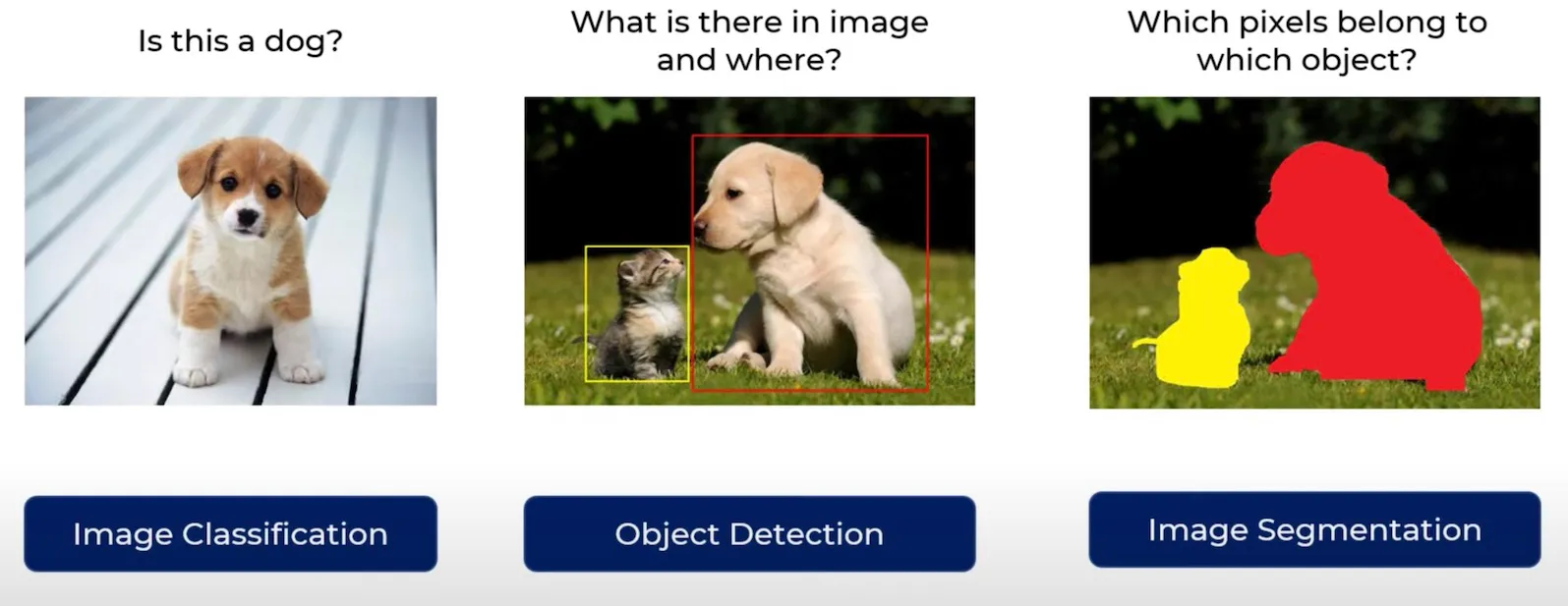
Classification vs detection vs segmentation (illustrative
example, source: kaggle.com).
Segmentation is a key technology in many domains:
- medical imaging (tumor and organ delineation),
- autonomous driving (road scene understanding),
- industrial inspection (finding defects),
- robotics (scene understanding and navigation),
- satellite and aerial image analysis (land cover mapping).
In this laboratory, you will move from global image‑level reasoning to dense prediction, where every pixel matters.
Goals
The objectives of this laboratory are to:
- understand the difference between classification, detection and semantic segmentation,
- learn how segmentation datasets are organized (images + pixel‑wise masks),
- implement and use a custom
Datasetand dataloaders for segmentation tasks, - build and train a simple convolutional encoder–decoder (U‑Net‑like) segmentation model in PyTorch,
- apply segmentation‑specific losses and metrics such as Dice and Intersection over Union (IoU),
- evaluate the model quantitatively and qualitatively by visualizing predicted masks,
- experiment with geometric data augmentations for segmentation.
Prerequisites
Install dependencies
PyTorch
pip3 install torch torchvision --index-url https://download.pytorch.org/whl/cu126Lightning
pip install lightningAdditional packages (optional but recommended)
pip install matplotlib pillowImports
Below is a typical set of imports you will need during this lab.
import os
from pathlib import Path

import lightning as L
import torch
import torch.nn as nn
import torch.nn.functional as F
from torch.utils.data import DataLoader, Dataset

from torchvision import transforms
from PIL import Image

import numpy as np
import matplotlib.pyplot as plt
Dataset
In this lab we will work with a binary foreground/background segmentation problem. Each input image has a corresponding mask of the same spatial size, where each pixel belongs to one of two classes:
0– background,1– object / foreground (region of interest).
Masks are stored as grayscale images: pixel values 0 and
255 (or another constant) are mapped to class indices
0 and 1. In practice, multi‑class segmentation
simply extends this idea to more labels.
A typical folder structure for a segmentation dataset looks like this:
data/
    train/
        images/
            image_0001.png
            image_0002.png
            ...
        masks/
            image_0001.png
            image_0002.png
            ...
    val/
        images/
        masks/
    test/
        images/
        masks/
Each image file in images/ has a corresponding mask in
masks/ with the same file name.
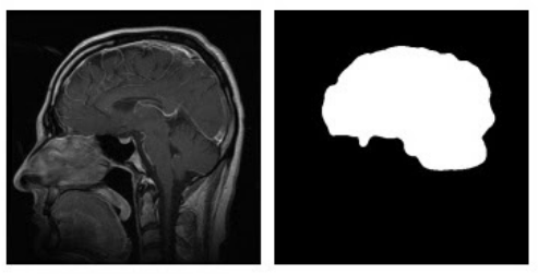
Example of an input image (left) and its corresponding
segmentation mask (right).
Segmentation fundamentals
Pixel‑wise classification view
Semantic segmentation can be seen as performing classification for each pixel independently, while also using information from surrounding pixels via convolutions.
For an image of size H × W and C classes,
the model outputs a tensor of shape:
(N, C, H, W)– for a batch ofNimages,
where each spatial position (h, w) has a vector of
C logits. After applying softmax over the
channel dimension, we obtain a probability distribution over classes for
every pixel.
The ground truth mask can be represented in two ways:
- Label map: tensor of shape
(N, H, W)with integer class indices, e.g.0– background,1– object. - One‑hot encoding: tensor of shape
(N, C, H, W)where each pixel is a one‑hot vector.
For most loss functions in PyTorch
(e.g. CrossEntropyLoss), we use the label map
representation.
Loss functions for segmentation
The simplest loss function is pixel‑wise cross‑entropy. For each pixel, we compute the cross‑entropy between the predicted class distribution and the true class, and then average over all pixels in the batch.
However, segmentation often suffers from class imbalance (few foreground pixels compared to background). In such cases, overlap‑based losses such as Dice loss are very popular.
The Dice coefficient for a single class is defined as:
\[ \text{Dice}(P, G) = \frac{2|P \cap G|}{|P| + |G|}, \]
where \(P\) is the set of predicted foreground pixels and \(G\) is the set of ground truth foreground pixels. The Dice loss is then:
\[ \mathcal{L}_{\text{Dice}} = 1 - \text{Dice}. \]
In practice, Dice can be computed in a differentiable way using probabilities or logits.
Metrics: IoU and Dice
To evaluate segmentation quality, we often report Intersection over Union (IoU) and Dice score.
For a given class, IoU is defined as:
\[ \text{IoU}(P, G) = \frac{|P \cap G|}{|P \cup G|}. \]
Dice and IoU are closely related; Dice tends to be slightly more forgiving for small objects.
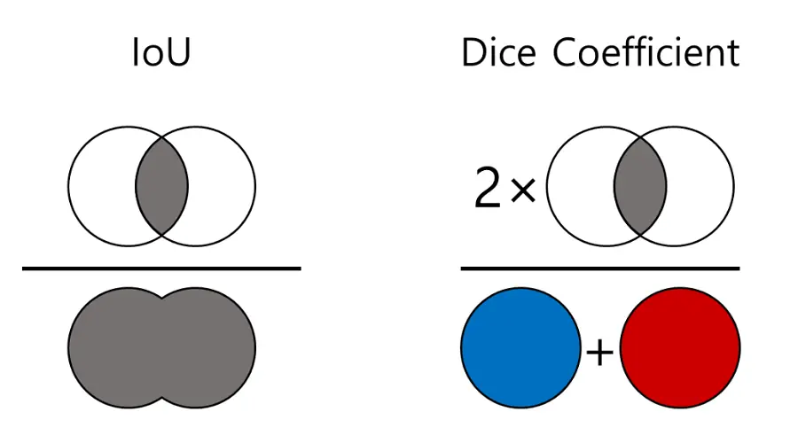
Comparison between Dice and Intersection over Union (IoU) – also
used in object detection.
For binary segmentation, we often report foreground Dice and foreground IoU. For multi‑class problems, we can compute these metrics per class and then average.
Segmentation model architectures
From classification CNNs to segmentation networks
In classification tasks, CNNs progressively downsample the feature maps using pooling or strided convolutions and finally apply a global pooling and a fully connected layer to produce a single prediction per image.
For segmentation, we need dense predictions with the same spatial resolution (or almost the same) as the input image. A common solution is to use an encoder–decoder architecture:
- the encoder is similar to a classification backbone (e.g. ResNet) and gradually reduces spatial resolution while increasing the number of feature channels,
- the decoder progressively upsamples feature maps back to the original resolution using transposed convolutions, bilinear upsampling, or interpolation,
- the final layer produces
num_classeschannels that represent per‑pixel logits.
U‑Net and skip connections
One of the most popular segmentation architectures is U‑Net. Its key idea is to combine coarse, high‑level features from deep layers with fine, high‑resolution features from shallow layers using skip connections.
The U‑Net consists of:
- Encoder (contracting path) – sequence of convolutional blocks and pooling operations.
- Decoder (expanding path) – upsampling layers that increase spatial resolution.
- Skip connections – feature maps from the encoder are concatenated with decoder features at matching resolutions, which helps recover fine details.
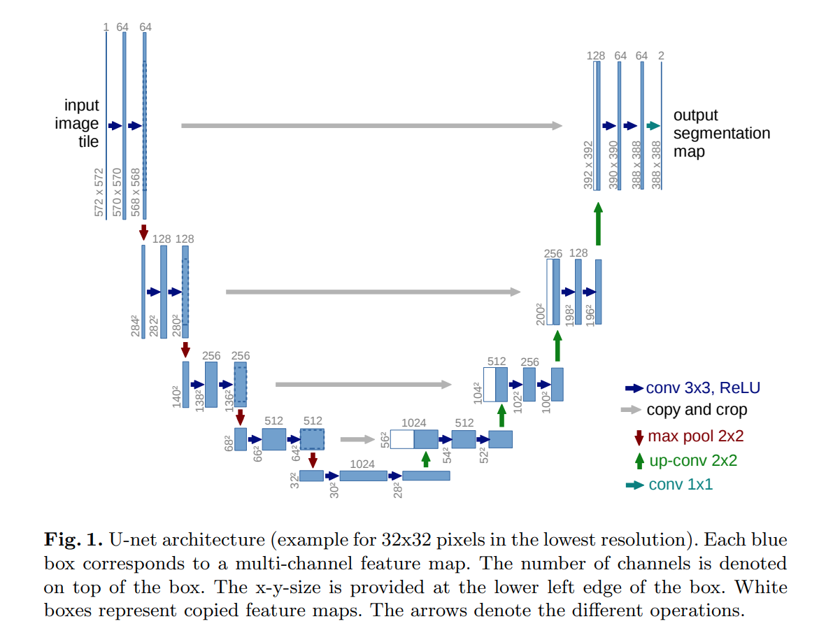
Simplified U‑Net style encoder–decoder architecture with skip
connections.
Note: In this lab, you will implement a small U‑Net‑like model from scratch.
Dataset and dataloaders
Segmentation dataset implementation
We start by implementing a custom PyTorch Dataset that
returns (image, mask) pairs for training.
class SegmentationDataset(Dataset):
    """Custom dataset for image segmentation.

    Each sample consists of an RGB image and a corresponding mask with
    integer labels (0 – background, 1 – foreground).
    """
    def __init__(self, images_dir: str, masks_dir: str, transform=None):
        self.images_dir = Path(images_dir)
        self.masks_dir = Path(masks_dir)
        self.transform = transform

        # Collect image paths and ensure masks exist
        self.image_paths = sorted(list(self.images_dir.glob("*.png")))
        if len(self.image_paths) == 0:
            raise RuntimeError(f"No images found in {self.images_dir}")

    def __len__(self) -> int:
        return len(self.image_paths)

    def __getitem__(self, idx: int):
        image_path = self.image_paths[idx]
        mask_path = self.masks_dir / image_path.name

        image = Image.open(image_path).convert("RGB")
        mask = Image.open(mask_path).convert("L")

        image = np.array(image)
        mask = np.array(mask)

        # Map mask to {0, 1}
        mask = (mask > 0).astype(np.uint8)

        if self.transform is not None:
            # Basic transform pipeline using torchvision transforms
            # We apply the same geometric transforms to image and mask
            augmented = self.transform(image=image, mask=mask)
            image = augmented["image"]
            mask = augmented["mask"]

        # Convert to tensors
        image = torch.from_numpy(image).permute(2, 0, 1).float() / 255.0
        mask = torch.from_numpy(mask).long()

        return image, mask
In practice, you can use libraries like
Albumentations to conveniently apply the same geometric
transforms to both images and masks. For simplicity, the example above
assumes a generic callable transform that returns a
dictionary with "image" and "mask" keys.
💥 Task 1 💥
Implement your own SegmentationDataset class based on
the template above. Make sure that:
- images are loaded as RGB and normalized to
[0, 1], - masks are loaded as single‑channel images and converted to integer
labels (
0/1), __getitem__returns(image_tensor, mask_tensor)with shapes(3, H, W)and(H, W).
Create training, validation and test datasets pointing to this dataset.
You will need to split the train folder into training and
validation sets (e.g. 80% train, 20% val).
Visualizing images and masks
Before training the model, it is very important to verify that images and masks are loaded correctly.
💥 Task 2 💥
Implement the visualization function to display a few random samples from your training dataset. Check that:
- masks are correctly aligned with images (no shifts or flips),
- foreground regions correspond to the expected objects.
If something looks wrong, fix your dataset implementation before continuing.
def show_samples(dataset, num_samples: int = 4):
    indices = np.random.choice(len(dataset), size=num_samples, replace=False)

    fig, axes = plt.subplots(2, num_samples, figsize=(4 * num_samples, 6))
    ############# TODO: Student code #####################
    for i, idx in enumerate(indices):
        pass

    ######################################################

    plt.tight_layout()
    plt.show()
Baseline segmentation model
U‑Net‑like architecture
In this section you will implement a simple U‑Net‑like encoder–decoder architecture. Below is a minimal implementation sketch of a U‑Net‑style network for binary segmentation.
class DoubleConv(nn.Module):
    """(Conv2d => ReLU) * 2 block."""
    def __init__(self, in_channels, out_channels):
        super().__init__()
        self.net = nn.Sequential(
            nn.Conv2d(in_channels, out_channels, kernel_size=3, padding=1),
            nn.BatchNorm2d(out_channels),
            nn.ReLU(inplace=True),
            nn.Conv2d(out_channels, out_channels, kernel_size=3, padding=1),
            nn.BatchNorm2d(out_channels),
            nn.ReLU(inplace=True),
        )

    def forward(self, x):
        return self.net(x)


class UNetSmall(nn.Module):
    def __init__(self, in_channels: int = 3, num_classes: int = 2):
        super().__init__()
        self.down1 = DoubleConv(in_channels, 64)
        self.down2 = DoubleConv(64, 128)
        self.down3 = DoubleConv(128, 256)

        self.pool = nn.MaxPool2d(2)

        self.bottleneck = DoubleConv(256, 512)

        self.up3 = nn.ConvTranspose2d(512, 256, kernel_size=2, stride=2)
        self.conv3 = DoubleConv(512, 256)

        self.up2 = nn.ConvTranspose2d(256, 128, kernel_size=2, stride=2)
        self.conv2 = DoubleConv(256, 128)

        self.up1 = nn.ConvTranspose2d(128, 64, kernel_size=2, stride=2)
        self.conv1 = DoubleConv(128, 64)

        self.head = nn.Conv2d(64, num_classes, kernel_size=1)

    def forward(self, x):
        ############# TODO: Student code #####################
        # Input -> Encoder -> Bottleneck -> Decoder with skip connections -> Final classification layer -> Output

        ######################################################
💥 Task 3 💥
Implement your own small U‑Net‑like architecture using the above sketch. Ensure that:
- the network takes input images of shape
(N, 3, H, W), - the output has shape
(N, num_classes, H, W)(no change in resolution), - skip connections from encoder to decoder are correctly implemented.
Test your model with a random input tensor and verify that shapes match.
Lightning module and training loop
To keep the training code clean and consistent with previous labs, we will wrap the segmentation model in a LightningModule.
💥 Task 4 💥
Create a training script (e.g. lab05.py) that:
- Creates dataloaders.
- Instantiates
LitSegmentationModel. - Creates a
Trainerand runs training and validation:trainer.fit(model, train_dataloaders=train_loader, val_dataloaders=val_loader). - Evaluates the model on the test set using
trainer.test.
Monitor training and validation loss. Verify that the model is able to overfit a very small subset of the training data (e.g. 10 images) as a sanity check.
Dice and IoU metrics
Dice score
Below is a simple implementation of the Dice score for binary segmentation.
def dice_score(preds: torch.Tensor, targets: torch.Tensor, eps: float = 1e-6) -> float:
    """Computes Dice score for binary segmentation.

    Parameters
    ----------
    preds : torch.Tensor
        Logits or probabilities with shape (N, 2, H, W) or predicted labels with shape (N, H, W).
    targets : torch.Tensor
        Ground truth labels with shape (N, H, W) where values are 0 or 1.
    """
    if preds.dim() == 4:
        preds = torch.argmax(preds, dim=1)

    preds = preds.float()
    targets = targets.float()

    intersection = (preds * targets).sum()
    union = preds.sum() + targets.sum()
    dice = (2.0 * intersection + eps) / (union + eps)
    return dice.item()
IoU
def iou_score(preds: torch.Tensor, targets: torch.Tensor, eps: float = 1e-6) -> float:
    if preds.dim() == 4:
        preds = torch.argmax(preds, dim=1)

    preds = preds.float()
    targets = targets.float()

    intersection = (preds * targets).sum()
    union = preds.sum() + targets.sum() - intersection
    iou = (intersection + eps) / (union + eps)
    return iou.item()
💥 Task 5 💥
Integrate Dice score and IoU
metrics into your LitSegmentationModel:
- compute Dice score and IoU in
training_step,validation_stepandtest_step, - log them using
e.g.
self.log("val_dice", dice, prog_bar=True)andself.log("val_iou", iou, prog_bar=True), - monitor how these metrics change over epochs.
Compare the behavior of Dice and IoU during training. Which one is more stable on your dataset?
Visualizing predictions
Numerical metrics are important, but for segmentation it is critical to look at the predicted masks.
@torch.no_grad()
def visualize_predictions(model, dataset, num_samples: int = 4, device: str = "cuda"):
    model.eval().to(device)

    indices = np.random.choice(len(dataset), size=num_samples, replace=False)
    fig, axes = plt.subplots(3, num_samples, figsize=(4 * num_samples, 8))

    for i, idx in enumerate(indices):
        image, mask = dataset[idx]
        image = image.to(device).unsqueeze(0)

        logits = model(image)
        preds = torch.argmax(logits, dim=1).squeeze(0).cpu()

        image_np = image.squeeze(0).cpu().permute(1, 2, 0).numpy()
        mask_np = mask.numpy()
        pred_np = preds.numpy()

        axes[0, i].imshow(image_np)
        axes[0, i].set_title("Image")
        axes[0, i].axis("off")

        axes[1, i].imshow(mask_np, cmap="gray")
        axes[1, i].set_title("Ground truth")
        axes[1, i].axis("off")

        axes[2, i].imshow(pred_np, cmap="gray")
        axes[2, i].set_title("Prediction")
        axes[2, i].axis("off")

    plt.tight_layout()
    plt.show()
💥 Task 6 💥
Use the visualization function above to inspect predictions on the validation or test set. Answer the following questions:
- Where does the model perform well? (large regions, clear boundaries, simple shapes)
- Where does it fail? (small objects, thin structures, noisy backgrounds)
- Are the predictions overly smooth or too noisy?
Experiment tracking
As in previous labs, you can use an experiment tracking tool (e.g. MLflow) to log:
- losses and metrics over time,
- hyperparameters (learning rate, batch size, augmentations),
- a few example predictions as images.
💥 Task 7 💥
Integrate experiment tracking into your training script and to facilitate comparison of different runs (with/without augmentations, different architectures, etc.).
Data augmentations for segmentation
In Lab 2 you worked with various image augmentations for classification (random crops, flips, color jitter, etc.). For segmentation, we must be more careful:
- geometric transforms (flip, rotate, crop, resize) must be applied jointly to the image and the mask,
- intensity transforms (brightness, contrast, blur, noise) are applied only to the image; the mask should remain unchanged.
Libraries like Albumentations provide convenient primitives for such joint transformations:
import albumentations as A
from albumentations.pytorch import ToTensorV2

train_transform = A.Compose([
    A.VerticalFlip(p=0.5),
    A.RandomResizeResizedCrop(height=256, width=256),
    A.ColorJitter(p=0.5),
    A.GaussianBlur(p=0.2),
    A.Normalize(),
    ToTensorV2(),
])
You can then pass this transform to SegmentationDataset
and use image / mask produced by
Albumentations directly.
💥 Task 8 💥
Add geometric augmentations to your training dataset. At minimum:
- random horizontal flip,
- random crop or random resized crop,
- random translation (10%),
- scaling (0.9, 1.1)
- optional rotation.
Train two models:
- without augmentations.
- with augmentations.
Compare Dice and IoU on the validation set and discuss the impact of augmentations on generalization.
Advanced usage
Transfer learning for segmentation
Instead of training the encoder from scratch, you can reuse a pretrained classification backbone (e.g. ResNet‑18) and attach a decoder on top.
💥 Task 9 💥
- replace the encoder part of your U‑Net with a pretrained backbone
from
torchvision.models, - freeze encoder weights for a few epochs, then unfreeze and fine‑tune,
- compare convergence speed and final metrics.
Ready-to-use segmentation models
You can also experiment with established segmentation architectures from libraries like Segmentation Models PyTorch (SMP).
pip3 install segmentation-models-pytorch💥 Task 10 💥
Use SMP to create a segmentation model (e.g. U‑Net with ResNet‑34 backbone) and train it on your dataset. Compare results with your custom implementation.
Multi‑class segmentation
If your dataset contains more than two classes, you can extend the model and metrics to multi‑class segmentation. To do this you should:
- modify your U‑Net to output
num_classeschannels, - adapt your loss function (use
CrossEntropyLosswith multi‑class masks or implement Dice loss), - compute Dice / IoU per class and mean them over classes.
💥 Task 11 💥
Find and download a segmentation dataset, for example from Kaggle Datasets, which has more than 2 classes and implement multi‑class segmentation.